|
We present here a web application for diffraction limited imaging parameters solution in paraxial space based on relations presented in paper: General relations for optical design parameters under diffraction limited paraxial imaging. Jan Hošek, Šárka Němcová, Vlastimil Havran, General relations for optical design parameters under diffraction limited paraxial imaging, Optics and Lasers in Engineering Volume 174, 107960 (2024). https://doi.org/10.1016/j.optlaseng.2023.107960 You can find the web application under link Web Application. If you have any questions or comments you can contact me on: Jan.Hosek@fs.cvut.cz |
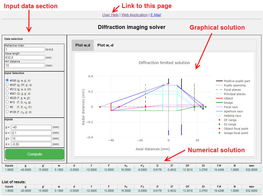
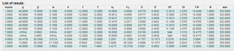
| We analyzed the fundamental relationships among general optical system parameters assuming a diffraction limited imaging in paraxial space. We discovered that the total twelve optical system parameters, which describe the optical imaging problem, are unambiguously determined by a set of four of these parameters under a diffraction condition. This condition is set so that the object image permitted blur is of the same size for both the spot due to defocus and the diffraction spot. There can be found, in total, 314 different optical system design approaches to fully describe the diffraction limited imaging problem. In our paper we presented eight of these design approaches. The Web Application allows the user to find diffraction limited imaging parameters according to the relations presented in the paper. It also shows a graphical solution for computed parameter's values. |
The Web Application window contains fields:
|
|
Input data section contains three input fields:
Enviroment
|
|
|
| g - object distance from the entrance pupil plane | g´ - image distance from the exit pupil plane | f - effective focal length in the object space | f´ - effective focal length in the image space | x0 - entrance pupil position from the front focal plane | x0´ - exit pupil position from the back focal plane | D - entrance pupil diameter | D´ - exit pupil diameter | w - object resolution limited by diffraction | d - image resolution limited by diffraction | DF - depth of field in the object space | DI - depth of focus in the image space | |
|
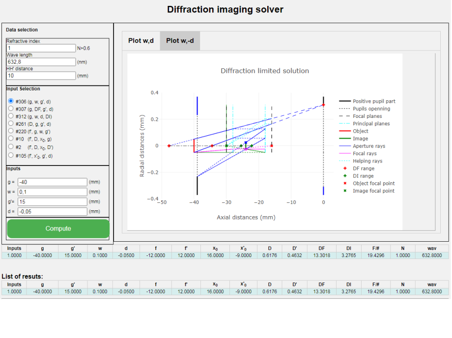
Results presentation section
Graphical solution
|
|
|
|
|
|
|
|
If you have any questions or comments you can contact me on: Jan.Hosek@fs.cvut.cz
Enjoy the app!